Feature Analysis of Defaulters in Credit Card Default problem

Creating models to predict credit card defaults can help financial institutions to make better decisions, reduce losses and improve their performance. Feature analysis is an important step after predicting credit card defaulters as it helps to understand the underlying reasons why certain customers are more likely to default, identify potential biases in the prediction model and ensure that the model is fair and equitable.

In this article, we will discuss the machine learning model (Random Forest), talk about a couple of tools that are used in feature analysis, and conclude our article with a Python code that applies the above concepts to a real dataset of credit card defaulters.

Random Forest Model

Random Forest is a popular machine learning algorithm that was first introduced in 2001 by Leo Breiman and Adele Cutler. It is an ensemble learning method that combines multiple decision trees to create a more robust and accurate model. The algorithm creates multiple decision trees by randomly selecting a subset of the data and a subset of the features to train each tree. The final prediction is made by averaging the predictions of all the decision trees.

The concept behind Random Forest is to reduce the variance of a single decision tree by averaging the predictions of multiple decision trees. This results in a model that is less prone to overfitting. Random Forest can be used for both classification and regression problems and is particularly useful for datasets with a large number of features.

Random Forest has many advantages, such as being easy to interpret and understand, being able to handle missing values, being robust to outliers, and being able to handle categorical features. However, Random Forest also has some disadvantages, such as being less interpretable than decision trees, being computationally intensive, and being less sensitive to small changes in the data.

The expensive computing in Random Forest comes from the creation of multiple decision trees. Each tree requires training on a subset of the data and a subset of the features, which can take a significant amount of time and computational resources, especially for large datasets with many features. Additionally, when making predictions, the algorithm must average the predictions of all the decision trees, which also requires significant computational resources.

Random Forest algorithm is widely used in many fields, such as finance, healthcare, and natural language processing. It’s also a popular method for feature selection and feature importance in order to understand the underlying factors that contribute to the prediction.

LIME

Local Interpretable Model-Agnostic Explanations (LIME) is a method for interpreting the predictions of any machine learning model. It was introduced in 2016 by Marco Tulio Ribeiro, Sameer Singh, and Carlos Guestrin. The concept behind LIME is to explain the predictions of a machine learning model by approximating it locally with a simpler interpretable model. In order to do this, LIME perturbs the input data and examines the effect on the model’s predictions. This is done by generating a set of simulated samples around the input and training a simple interpretable model on the set of simulated samples and their corresponding predictions. LIME then uses this interpretable model to explain the predictions of the original model.

One of the main advantages of LIME is that it is model-agnostic, meaning it can be used to explain the predictions of any machine learning model, regardless of its complexity. Additionally, LIME can provide explanations for individual predictions, which can be useful for understanding why a model made a particular prediction. LIME also allows the creation of perturbations that are tailored to the input data, which can be useful for understanding the features that have a higher importance in the model decision.

However, LIME also has some disadvantages. One of the main limitations is that it can be computationally expensive, especially for large datasets or high-dimensional data. Additionally, LIME can be sensitive to the choice of interpretable model and the number of perturbations used, which can affect the quality of the explanations. The interpretable model choice is a trade-off between the simplicity of the model and the accuracy of the explanations. The number of perturbations can also affect the quality of the explanations and the computational cost.

Eli5

Eli5 (Explain like I’m 5) is an open-source library for model interpretability and feature selection. It was introduced in 2015 and is built on top of the popular machine learning library scikit-learn. The concept behind Eli5 is to provide easy-to-understand explanations for the predictions of machine learning models.

One of the main advantages of Eli5 is its simplicity and ease of use. It provides a user-friendly interface for interpreting the predictions of machine learning models and can be easily integrated into any scikit-learn workflow. Additionally, Eli5 can be used to analyze the feature importance of a model, which can be useful for feature selection and understanding the underlying factors that contribute to the predictions.

However, Eli5 is designed to be used with scikit-learn models, so it may not be compatible with other machine learning libraries. Additionally, it can be less flexible than other interpretability tools and may not work well for models with high-dimensional data.

Eli5 is widely used in many fields, such as natural language processing, computer vision, healthcare, and finance. It’s particularly useful for creating interpretable models for non-technical users, it can be used to explain the predictions of a credit risk model, which can help to understand the underlying factors that contribute to credit card default and ensure that the model is fair and equitable.

Feature Analysis using Python

In this section, we will use a credit card dataset, build a Random Forest model to predict the defaulters, then interpret the model using LIME and Eli5.

We will start by importing the necessary libraries:

import numpy as np import pandas as pd import matplotlib.pyplot as plt import seaborn as sns from sklearn.model_selection import train_test_split from sklearn.model_selection import RandomizedSearchCV from sklearn.ensemble import RandomForestClassifier import sklearn.metrics as metrics from sklearn.metrics import confusion_matrix from sklearn.metrics import classification_report import lime import lime.lime_tabular

Then we will read the data:

data = pd.read_csv(“./Credit_Card.csv”) data.info()

<class ‘pandas.core.frame.DataFrame’>

RangeIndex: 30000 entries, 0 to 29999

Data columns (total 25 columns):

 #   Column                      Non-Null Count  Dtype  

—  ——                      ————–  —–  

 0   ID                          30000 non-null  int64  

 1   LIMIT_BAL                   30000 non-null  float64

 2   SEX                         30000 non-null  int64  

 3   EDUCATION                   30000 non-null  int64  

 4   MARRIAGE                    30000 non-null  int64  

 5   AGE                         30000 non-null  int64  

 6   PAY_1                       30000 non-null  int64  

 7   PAY_2                       30000 non-null  int64  

 8   PAY_3                       30000 non-null  int64  

 9   PAY_4                       30000 non-null  int64  

 10  PAY_5                       30000 non-null  int64  

 11  PAY_6                       30000 non-null  int64  

 12  BILL_AMT1                   30000 non-null  float64

 13  BILL_AMT2                   30000 non-null  float64

 14  BILL_AMT3                   30000 non-null  float64

 15  BILL_AMT4                   30000 non-null  float64

 16  BILL_AMT5                   30000 non-null  float64

 17  BILL_AMT6                   30000 non-null  float64

 18  PAY_AMT1                    30000 non-null  float64

 19  PAY_AMT2                    30000 non-null  float64

 20  PAY_AMT3                    30000 non-null  float64

 21  PAY_AMT4                    30000 non-null  float64

 22  PAY_AMT5                    30000 non-null  float64

 23  PAY_AMT6                    30000 non-null  float64

 24  default.payment.next.month  30000 non-null  int64  

dtypes: float64(13), int64(12)

memory usage: 5.7 MB

We see that the file has 30.000 entries and 25 columns. There are no null values according to the data info.
The dataset contains information on 30.000 credit card holders. Some of its features are: given credit, sex, education level, marital status, age, the past 6 months’ payment and billing details, and finally the target feature “default payment next month”. 

After studying the dataset, we can do some cleaning in Education and Marriage features, to help the model give better predictions.
We will reduce the Education feature into graduate school(1), high school(2), university(3), and others(4).
And we’ll reduce the options of Marriage into married(1), single(2), or others(3).

data[‘EDUCATION’]=np.where(data[‘EDUCATION’] == 5, 4, data[‘EDUCATION’]) data[‘EDUCATION’]=np.where(data[‘EDUCATION’] == 6, 4, data[‘EDUCATION’]) data[‘EDUCATION’]=np.where(data[‘EDUCATION’] == 0, 4, data[‘EDUCATION’]) data[‘MARRIAGE’]=np.where(data[‘MARRIAGE’] == 0, 3, data[‘MARRIAGE’])

Splitting the data into features and target, then splitting it again into the training set and testing set, and storing the names of the features in a list:

X = data.drop(‘default.payment.next.month’,axis=1) Y = data[‘default.payment.next.month’] x_train,x_test,y_train,y_test = train_test_split(X,Y,train_size=0.85,random_state=42) feature_names = (x_train.columns)

Tuning the Random Forest, so we get the best accuracy. 

param_dist = {‘n_estimators’: [50,100,150,200,250,300], #trees in the forest           “max_features”: [1,2,3,4,5,6,7,8,9,10,11,12], #features to be considered           ‘max_depth’: [1,2,3,4,5,6,7,8,9,10,11,12], #max depth of the tree           “criterion”: [“gini”, “entropy”]} #measure the quality of the split rf = RandomForestClassifier() rf_cv = RandomizedSearchCV(rf, param_distributions = param_dist,                       cv = 5, random_state=0, n_jobs = -1) rf_cv.fit(x_train, y_train) print(“Tuned Random Forest Parameters: %s” % (rf_cv.best_params_))

Tuned Random Forest Parameters: {‘n_estimators’: 100, ‘max_features’: 11, ‘max_depth’: 4, ‘criterion’: ‘gini’}

We take the best parameters according to our tuning, and build the Random Forest depending on these parameters:

tuned_rf = RandomForestClassifier(criterion= ‘gini’, max_depth= 4,                                 max_features= 11, n_estimators= 100,                                 random_state=0) tuned_rf.fit(x_train, y_train) y_pred = tuned_rf.predict(x_test) print(‘Accuracy:’, metrics.accuracy_score(y_pred,y_test))

Accuracy: 0.8206666666666667

We got an accuracy of 82 percent. It is an acceptable accuracy. However, you can get better results if you do better cleaning of the data or try every possible parameter while tuning the forest.
We will accept the 82 percent accuracy for now.

Now it is time to plot a confusion matrix of the results:

plt.figure(figsize=(8,6),dpi=300) ConfMatrix = confusion_matrix(y_test,tuned_rf.predict(x_test)) sns.heatmap(ConfMatrix,annot=True, cmap=“Blues”, fmt=“d”,         xticklabels = [‘Non-default’, ‘Default’],         yticklabels = [‘Non-default’, ‘Default’]) plt.ylabel(‘True label’) plt.xlabel(‘Predicted label’) plt.title(“Confusion Matrix – Random Forest”)

Applying LIME on a couple of defaulters’ rows to find out the relationship between different features and the target feature:

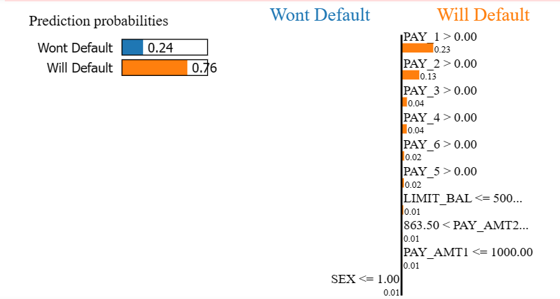
predict_fn_rf = lambda x: tuned_rf.predict_proba(x).astype(float) explainer = lime.lime_tabular.LimeTabularExplainer(x_train.values, feature_names=feature_names, class_names=[‘Won’t Default’,‘Will Default’], verbose=False, mode=‘classification’) choosen_instance = X.iloc[[18256]].values[0] exp = explainer.explain_instance(choosen_instance, predict_fn_rf, num_features=10) exp.show_in_notebook(show_table=True)

choosen_instance = X.iloc[[0]].values[0] exp = explainer.explain_instance(choosen_instance, predict_fn_rf, num_features=10) exp.show_in_notebook(show_table=True)

As we see, in the two random defaulters we analyzed, ‘PAY_1’ and ‘PAY_2’ features are crucial in determining whether someone is gonna default or not.

Now let’s apply Eli5:

import eli5 eli5.show_weights(tuned_rf,top=10)

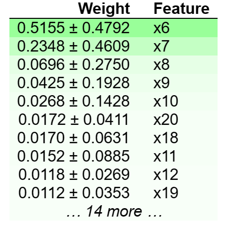
We see again that columns number 6, 7, 8, 9, and 10 (PAY_1 -> PAY_5) are the most important features to determine whether someone will default or not. These columns represent the repayment status in the last 5 months. 

Final Words

In conclusion, this article has discussed the use of Random Forest, LIME, and Eli5. These tools can be used to gain insights into the workings of a machine learning model and can be especially useful when working with complex models such as Random Forest. The practical part of the article demonstrated the application of these tools in building a model and interpreting its results. However, it is important to note that there are other interpretability tools available, such as SHAP, that can also be used to gain a further understanding of a model’s behavior. Overall, the use of interpretability tools is an important step in the development of any machine learning model, as it can help to ensure that the model is behaving as expected and that its predictions are trustworthy.